Apply SciPy's correlate() to the waveformswaveforms of antenna pairsantenna pairs to determine incoming signal directions. More...

Functions
pl.DataFrame	supply_azimuthal_angle_masks (pl.DataFrame skymaps)
	Supplies azimuth masks to any sky map (eg time delay mapstime delay maps or correlation mapscorrelation maps).
pl.DataFrame	combine_time_delay_maps_and_waveforms (pl.DataFrame masks_and_skymaps, pl.DataFrame waveforms)
	Prepares a big table that has all the column needed by cross_correlate.
pl.DataFrame	cross_correlate (pl.DataFrame big_frame)
	Compute the zero-centered normalized cross correlation (ZNCC) and makes correlation skymaps.
[float, float]	_get_true_direction (ROOT.pueo.Dataset dataset)
	Returns the true signal direction.
None	plot_correlation_map (pl.DataFrame correlation_frame, str plot_name, true_phi=None, true_theta=None)
	Plots the reult of cross_correlate.

Detailed Description

Apply SciPy's correlate() to the waveformswaveforms of antenna pairsantenna pairs to determine incoming signal directions.

Function Documentation

◆ supply_azimuthal_angle_masks()

pl.DataFrame supply_azimuthal_angle_masks ( pl.DataFrame skymaps )

Supplies azimuth masks to any sky map (eg time delay mapstime delay maps or correlation mapscorrelation maps).

Parameters

[in] skymaps columns A1_PhiSector and A2_PhiSector are required

Return values

phi_masks see the schema of the example output below

Parameters:
- Input: required columns are the $\phi$-sectors of the antenna pairs, A1_PhiSector and A2_PhiSector.
- Output schema: one column (masks) will be attached to the input dataframe,
  $ A1_PhiSector <u8>
  
  $ A2_PhiSector <u8>
  
  $ masks <array[bool, (1, 360)]>
Explanation:
- $\phi$-sector 1 is centered around 0 degrees azimuth, $\phi$-sector 2 around 15 degrees, and so on and so forth; the last $\phi$ sector (24) is centered around 345 degrees.
- Based on the antenna's field of viewfield of view

, the values outside a certain range are dropped.

In the figure below, we show what this would look like for antennas from the first three and the last $\phi$-sectors (white means masked).

Example masks of a few phi-sectors

The chosen masking behavior for now is that only the data within the overlapping unmasked range would be kept.
For instance, suppose an antenna from $\phi$-sector 1 is paired with an antenna from $\phi$-sector 2, then:

Example superimposed masks

Warning

Thus, if the antenna pair's fields of viewfields of view

do not overlap, then everything will be masked.

Definition at line 34 of file locate_signal.py.

◆ combine_time_delay_maps_and_waveforms()

pl.DataFrame combine_time_delay_maps_and_waveforms	(	pl.DataFrame	masks_and_skymaps,
		pl.DataFrame	waveforms )

Prepares a big table that has all the column needed by cross_correlate.

Parameters

[in]	masks_and_skymaps	The output of supply_azimuthal_angle_masks
[in]	waveforms	The output of waveform_plots.load_waveforms

Return values

big_frame See sample output schema below.

Parameters:
- The following columns are required in waveforms:
  1. AntNum
  2. waveforms (volts)
  3. step size (nanoseconds)
  4. Pol
- The following columns are required in masks_and_skymaps:
  1. A1_AntNum
  2. A2_AntNum
  3. time delays [sec]
  4. masks
- The output schema:
  $ A1_AntNum <enum>
  
  $ A2_AntNum <enum>
  
  $ Pol <enum>
  
  $ A1_waveforms (volts) <array[f64, 3072]>
  
  $ A2_waveforms (volts) <array[f64, 3072]>
  
  $ time delays [samples] <array[i64, (180, 360)]>
  
  $ masks <array[bool, (1, 360)]>
Explanation:
- time delays [samples] refers to the time delay skymapstime delay skymaps

, with the units converted from seconds to "samples"

That is, the units are in "steps" (step size (nanoseconds))
The values in these time delay skymaps are therefore integers, serving as indices.
These indices are then used later in cross_correlate when creating the correlation skymaps based on the time delay maps (via "fancy-indexing").
Qualitatively, the time delay maps have not changed. For example:

Time Delay Map in Seconds

Time Delay Map in Samples

Definition at line 149 of file locate_signal.py.

◆ cross_correlate()

pl.DataFrame cross_correlate ( pl.DataFrame big_frame )

Compute the zero-centered normalized cross correlation (ZNCC) and makes correlation skymaps.

Parameters

[in] big_frame The output of combine_time_delay_maps_and_waveforms()

Return values

correlation_maps See the schema of the example output below

Parameters: columns correlation and correlation maps will be added to the input, so the output schema looks like
$ A1_AntNum <enum>

$ A2_AntNum <enum>

$ Pol <enum>

$ A1_waveforms (volts) <array[f64, 3072]>

$ A2_waveforms (volts) <array[f64, 3072]>

$ time delays [samples] <array[i64, (180, 360)]>

$ masks <array[bool, (1, 360)]>

$ correlation <array[f64, 6143]>

$ correlation maps <array[f64, (180, 360)]>
- correlation maps contain correlation skymaps. These are matrices with the same dimensions as the time delay maps of time delays [samples], as the former are made based on the latter via "fancy-indexing"
- Each matrix element of a correlation skymap is the correlation score between two waveforms, given some particular time delaytime delay

, ie. phase shift.

masks can be used to mask the correlation maps, as shown in the bottom subplot in the Figure above. The masks are defined by supply_azimuthal_angle_masks.

Explanation:
- Consider two waveforms,
- Each row in the correlation column is an array of correlation scores.
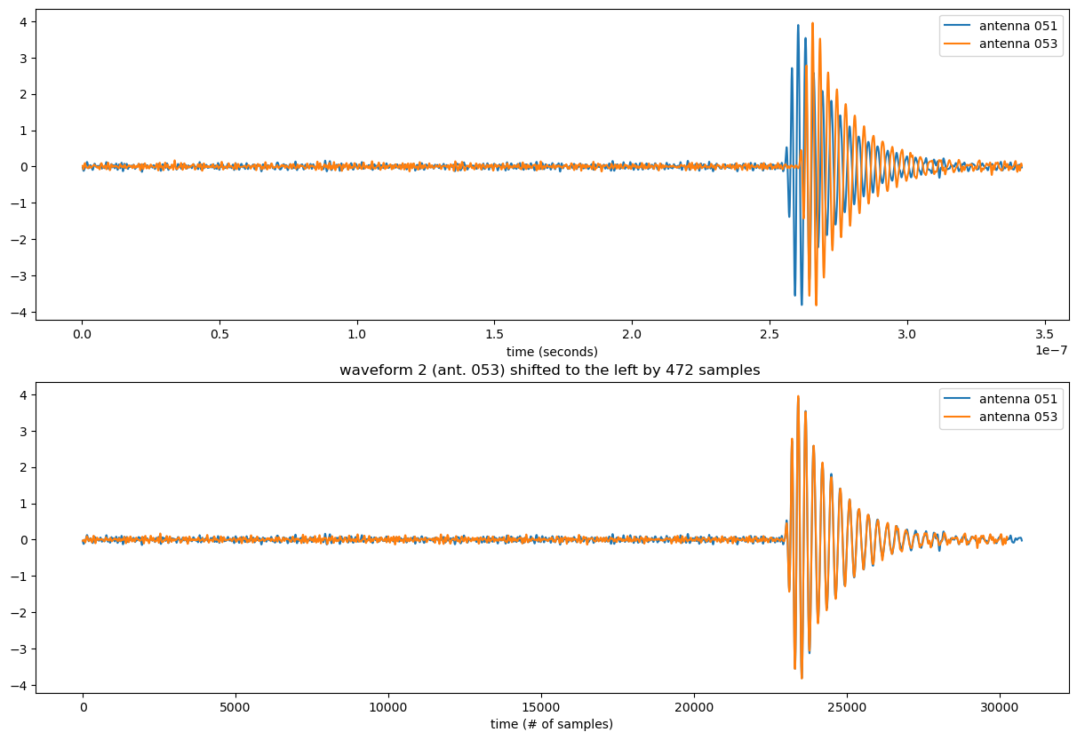
- By shifting the waveforms we may be able to get them to align perfectly, at which point maximum correlation is achieved.
- The correlation score tells us how "aligned" the two waveforms are after we phase shift A1_waveforms (volts) against A2_waveforms (volts) by a certain amount of time.
- The waveforms are zero-centered and normalized such that the cross-correlation is bounded between [-1,1]. Zero means the waveforms are not aligned at all.
- See cross_correlation_and_time_delay.pdf or, for details, scipy_correlate_behavior.pdf.

Definition at line 217 of file locate_signal.py.

◆ _get_true_direction()

[float, float] _get_true_direction ( ROOT.pueo.Dataset dataset )

protected

Returns the true signal direction.

Parameters

[in] dataset The output of initialise.load_pueoEvent_Dataset

Note that as stored in the .root files, the variable RFdir_payload is the direction the signal is travelling to.
Therefore, to obtain the direction that the signal is coming from, we need the opposite vector.
Thus, $\phi_{\rm true} = (\phi_{\rm rfdir} + 180 ^\circ) \% 360^\circ$, and $\theta_{\rm true} = 180^\circ - \theta_{\rm rfdir}$

Definition at line 299 of file locate_signal.py.

◆ plot_correlation_map()

None plot_correlation_map	(	pl.DataFrame	correlation_frame,
		str	plot_name,
			true_phi = None,
			true_theta = None )

Plots the reult of cross_correlate.

Parameters

[in]	correlation_frame	The output of cross_correlate
[in]	plot_name	Remember to specify file type
[in]	true_phi	(optional) from _get_true_direction
[in]	true_theta	(optional) from _get_true_direction

Required columns in correlation_frame:
1. correlation maps
2. masks
3. Pol
Using only one antenna pair, one can find a band of peak correlation scores, see the plot in the file description.
If we then sum over all antenna pairs, we would be able to identify a single peak:

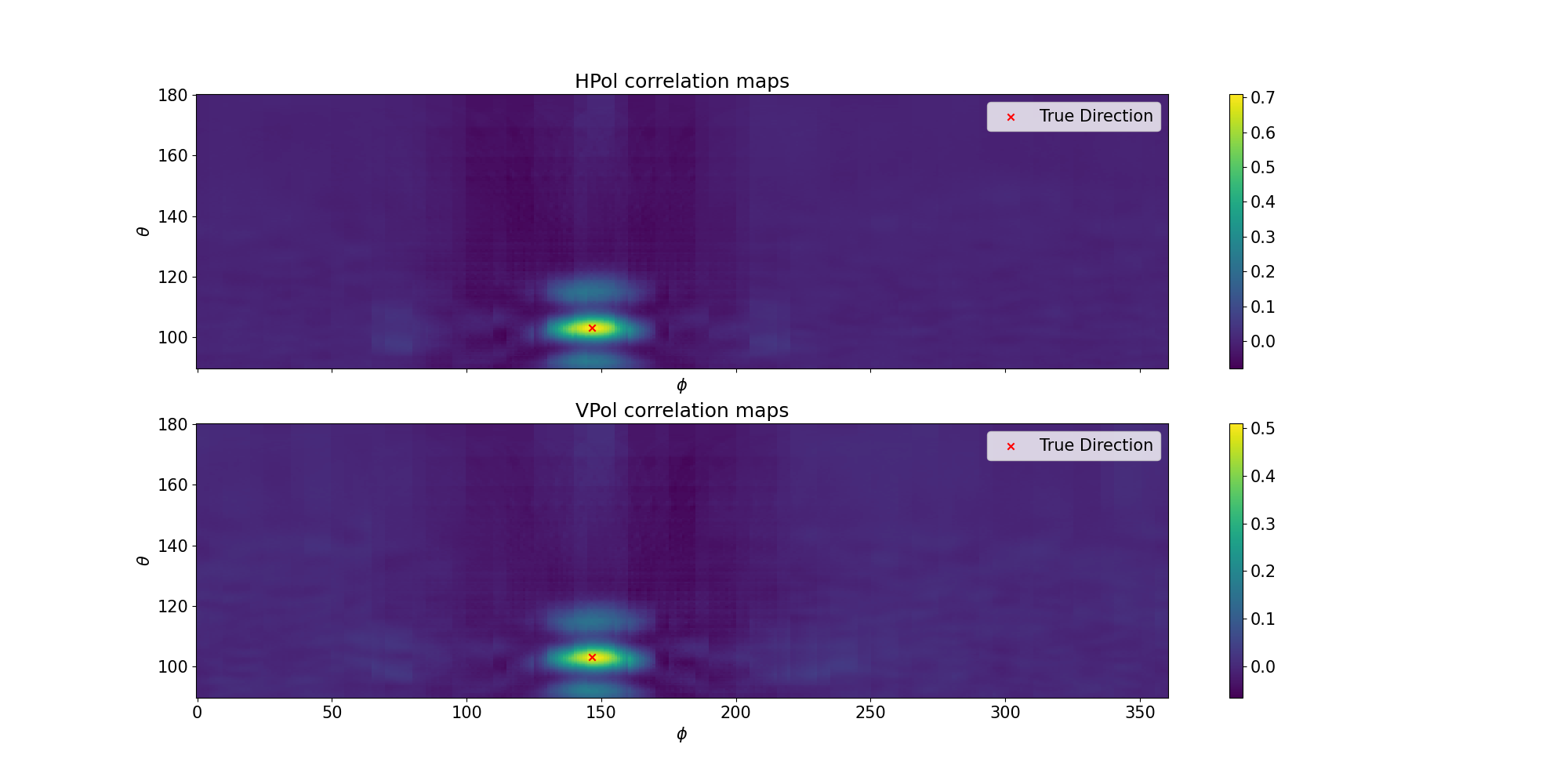
Correlation Skymaps (summed over all antenna pairs)

Definition at line 319 of file locate_signal.py.

Functions

Detailed Description

Function Documentation

◆ supply_azimuthal_angle_masks()

◆ combine_time_delay_maps_and_waveforms()

◆ cross_correlate()

◆ _get_true_direction()

◆ plot_correlation_map()