locate_signal.py

Go to the documentation of this file.

r"""!
@file  locate_signal.py
@brief `main()` shows how to use [cross_correlate()](#locate_signal.cross_correlate)
and [plot_correlation_map()](#locate_signal.plot_correlation_map).
 
\anchor example_one_pair_corr_map
![Unmasked and Masked Correlation Maps: one antenna pair](example_correlation_map_one_pair.png)
 
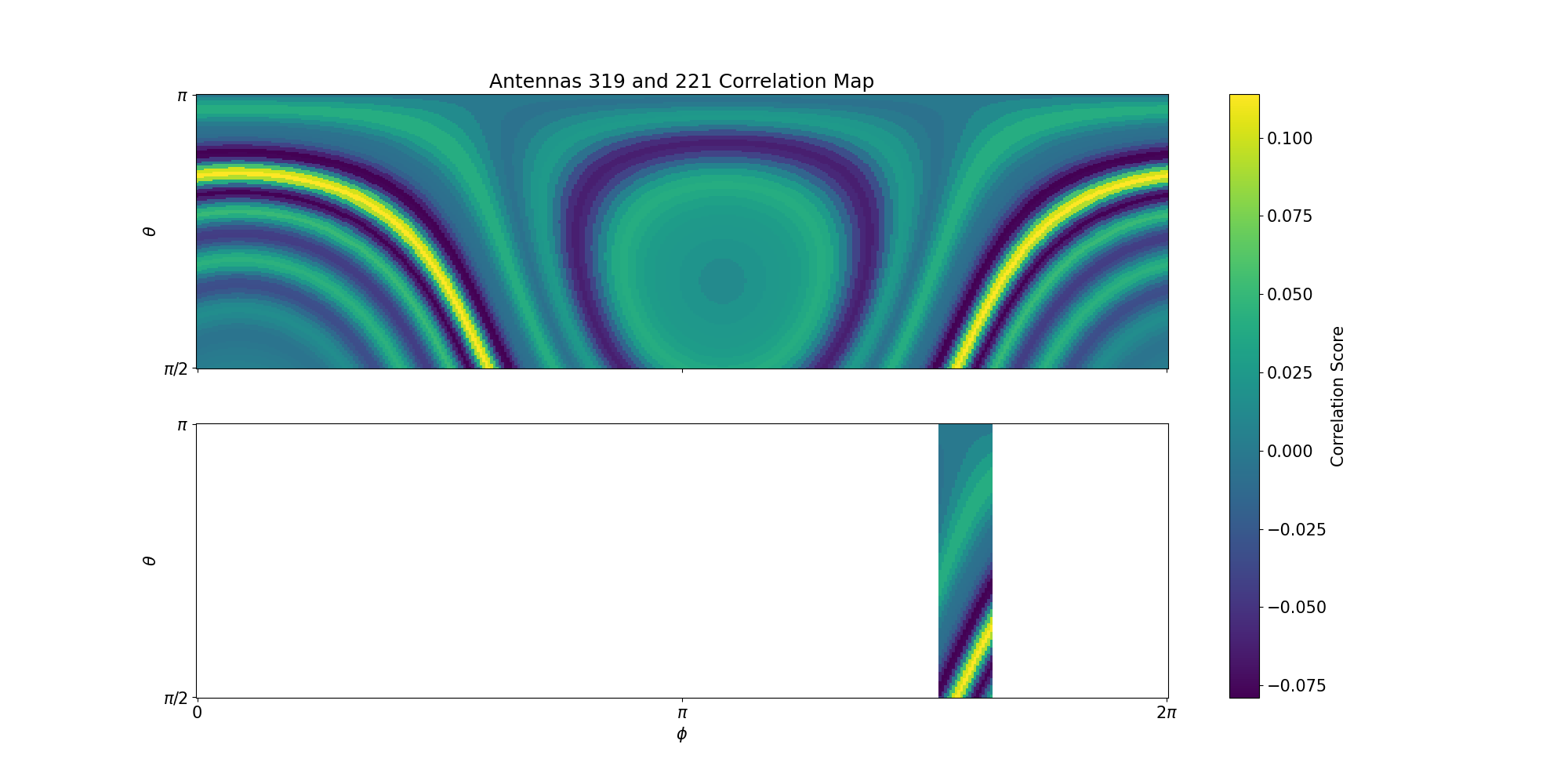
Summing over all antenna pairs, we have
 
\anchor example_corr_map
![Unmasked and Masked Total Correlation Maps](example_correlation_map_2D.png)
 
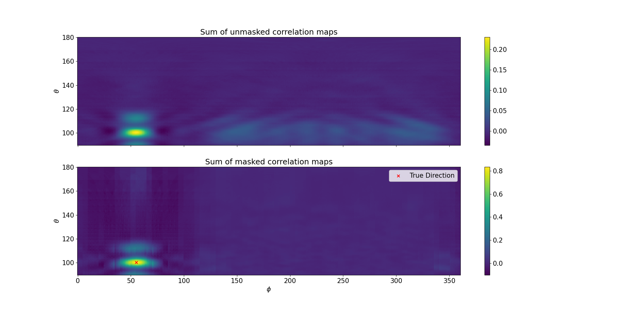
We can see that by masking the individual correlation maps, the total correlation map is less
noisy.
 
"""
 
import ROOT
import numpy as np
import polars as pl
from time_delays import _make_grid
from pathlib import Path
from initialise import load_pueoEvent_Dataset
 

 
 
def supply_azimuthal_angle_masks(skymaps: pl.DataFrame) -> pl.DataFrame:
    r"""!Supplies azimuth masks to any sky map
    (eg [time delay maps](#time_delays.make_time_delay_skymap) or
    [correlation maps](#cross_correlate))
    @ingroup CC
    @param[in]  skymaps        columns `A1_PhiSector` and `A2_PhiSector` are **required**
    @retval     phi_masks      see the schema of the example output below
 
* Parameters:
    *   Input: required columns are the \f$\phi\f$-sectors of the antenna pairs,
        `A1_PhiSector` and `A2_PhiSector`.
    *   Output schema: one column (`masks`) will be attached to the input dataframe,
```
$ A1_PhiSector                    <u8>
$ A2_PhiSector                    <u8>
$ masks        <array[bool, (1, 360)]>
```
 
* Explanation:
 
    * \f$\phi\f$-sector 1 is centered around 0 degrees azimuth, \f$\phi\f$-sector 2 around 15 degrees,
      and so on and so forth; the last \f$\phi\f$ sector (24) is centered around 345 degrees.
    * Based on the antenna's [field of view](#antenna_attributes.ASSUMED_PHI_SECTOR_APERTURE_WIDTH),
      the values outside a certain range are dropped.
    * In the figure below, we show what this would look like for antennas from the first three and
      the last \f$\phi\f$-sectors (white means masked).
 
      ![Example masks of a few phi-sectors](azimuthal_angle_masks_illustration.svg)
 
    * The chosen masking behavior for now is that **only the data within the overlapping unmasked
      range would be kept**.
    * For instance, suppose an antenna from \f$\phi\f$-sector 1 is paired with an antenna from
      \f$\phi\f$-sector 2, then:
 
      ![Example superimposed masks](azimuthal_angle_mask_overlap_illustration.svg)
 
    @warning
    * Thus, if the antenna pair's
      [fields of view](#antenna_attributes.ASSUMED_PHI_SECTOR_APERTURE_WIDTH)
      do not overlap, then everything will be masked.
    """
    from antenna_attributes import NUM_PHI_SECTORS, ASSUMED_PHI_SECTOR_APERTURE_WIDTH
    phi, _ = _make_grid(sparse=True)
    phi = np.degrees(phi)
 
    # eg. PhiSector 1 is centered around 0, so with aperture width 50 degrees,
    #     its bound would be (-25, 25)
    aperture_bounds = (
        pl.DataFrame(
            {"PhiSector": np.arange(1, 25)}, schema={"PhiSector": pl.UInt8}
        )
        .with_columns
        (
            ((pl.col("PhiSector") - 1) * (360 / NUM_PHI_SECTORS)).alias("aperture center [deg]")
        )
        .with_columns
        (
            pl.col("aperture center [deg]"),
            (
                (pl.col("aperture center [deg]") - ASSUMED_PHI_SECTOR_APERTURE_WIDTH / 2)
            ).alias("left bound [deg]"),
            (
                (pl.col("aperture center [deg]") + ASSUMED_PHI_SECTOR_APERTURE_WIDTH / 2)
            ).alias("right bound [deg]"),
        )
    )
 
    phi_masks = (
        skymaps
        .join(
            aperture_bounds.select(
                pl.col("PhiSector"),
                pl.col("left bound [deg]").alias("A1 left"),
                pl.col("right bound [deg]").alias("A1 right"),
            ), left_on="A1_PhiSector", right_on="PhiSector"
        ).join(
            aperture_bounds.select(
                pl.col("PhiSector"),
                pl.col("left bound [deg]").alias("A2 left"),
                pl.col("right bound [deg]").alias("A2 right"),
            ), left_on="A2_PhiSector", right_on="PhiSector"
        ).with_columns(
            pl.struct(pl.col("A1 left"), pl.col("A1 right"))
            .map_batches
            (
                lambda s: np.array([
                    ((phi - left) % 360) < ((right - left) % 360)
                    for left, right
                    in s.to_numpy()
                ])
            ).alias("A1 masks"),
            pl.struct(pl.col("A2 left"), pl.col("A2 right"))
            .map_batches
            (
                lambda s: np.array([
                    ((phi - left) % 360) < ((right - left) % 360)
                    for left, right
                    in s.to_numpy()
                ])
            ).alias("A2 masks")
        )
        .select(
            pl.all().exclude(
                "A1 masks", "A2 masks", "A1 left", "A2 left", "A1 right", "A2 right"
            ),
            pl.struct("A1 masks", "A2 masks").map_batches(
                lambda s: np.array([  # note: only overlapping part is kept, hence the element-wise &
                    ~(m1 & m2) for m1, m2 in s.to_numpy()
                ])  # the not (~) is used since True means masked in NumPy.
            ).alias("masks")
        )
    )
    return phi_masks
 
 
def combine_time_delay_maps_and_waveforms(masks_and_skymaps: pl.DataFrame,
                                          waveforms: pl.DataFrame) -> pl.DataFrame:
    r"""!Prepares a big table that has all the column needed by #cross_correlate.
    @ingroup CC
    @param[in]  masks_and_skymaps  The output of #supply_azimuthal_angle_masks
    @param[in]  waveforms          The output of #waveform_plots.load_waveforms
    @retval     big_frame          See sample output schema below.
 
    * Parameters:
        *   The following columns are required in `waveforms`:
            -#  `AntNum`
            -#  `waveforms (volts)`
            -#  `step size (nanoseconds)`
            -#  `Pol`
        *   The following columns are required in `masks_and_skymaps`:
            -#  `A1_AntNum`
            -#  `A2_AntNum`
            -#  `time delays [sec]`
            -#  `masks`
        *   The output schema:
```
$ A1_AntNum                               <enum>
$ A2_AntNum                               <enum>
$ Pol                                     <enum>
$ A1_waveforms (volts)        <array[f64, 3072]>
$ A2_waveforms (volts)        <array[f64, 3072]>
$ time delays [samples] <array[i64, (180, 360)]>
$ masks                  <array[bool, (1, 360)]>
```
    * Explanation:
        * `time delays [samples]` refers to the [time delay skymaps](#time_delays.make_time_delay_skymap),
          with the units converted from seconds to "samples"
        * That is, the units are in "steps" (`step size (nanoseconds)`)
        * The values in these time delay skymaps are therefore integers, serving as indices.
        * These indices are then used later in #cross_correlate when creating the
          correlation skymaps based on the time delay maps (via "fancy-indexing").
        * Qualitatively, the time delay maps have not changed. For example:
          \image html time_delay_map_in_seconds.svg  Time Delay Map in Seconds  width=40%
          \image html time_delay_map_in_samples.svg  Time Delay Map in Samples  width=40%
    """
 
    signal_length = len(waveforms["waveforms (volts)"][0])
    step_size = waveforms["step size (nanoseconds)"][0] * 1e-9  # ns -> seconds
 
    big_frame = (
        masks_and_skymaps
        .join(waveforms, left_on="A1_AntNum", right_on="AntNum")
        .join(waveforms, left_on=["A2_AntNum", "Pol"], right_on=["AntNum", "Pol"])
        .with_columns(
            (  # Convert [sec] to [number of samples]
                pl.col("time delays [sec]") / step_size + signal_length - 1
               # This offset is related to scipy.signal.correlate's behavior.
            )  # Next, round the time delay maps to integers.
            .map_batches(lambda s: np.rint(s.to_numpy()).astype(int))
            .alias("time delays [samples]")
        )
        .with_columns(
            pl.col("waveforms (volts)").alias("A1_waveforms (volts)"),
            pl.col("waveforms (volts)_right").alias("A2_waveforms (volts)")
        )
        .select(
            r"^A[12]_AntNum$", "Pol", r"^A[12]_waveforms \‍(volts\‍)$", "time delays [samples]", "masks"
        )
    )
 
    return big_frame
 
 
def cross_correlate(big_frame: pl.DataFrame) -> pl.DataFrame:
    r"""!Compute the zero-centered normalized cross correlation (ZNCC) and makes correlation skymaps
    @ingroup CC
    @param[in]  big_frame        The output of #combine_time_delay_maps_and_waveforms()
    @retval     correlation_maps See the schema of the example output below
 
    *   Parameters: columns `correlation` and `correlation maps` will be added to the input,
        so the output schema looks like
```
$ A1_AntNum                               <enum>
$ A2_AntNum                               <enum>
$ Pol                                     <enum>
$ A1_waveforms (volts)        <array[f64, 3072]>
$ A2_waveforms (volts)        <array[f64, 3072]>
$ time delays [samples] <array[i64, (180, 360)]>
$ masks                  <array[bool, (1, 360)]>
$ correlation                 <array[f64, 6143]>
$ correlation maps      <array[f64, (180, 360)]>
```
        *   `correlation maps` contain correlation skymaps.
            These are matrices with the same dimensions as the time delay maps of `time delays [samples]`,
            as the former are made based on the latter via "fancy-indexing"
 
        *   Each matrix element of a correlation skymap is the correlation score between two waveforms,
            given some particular [time delay](#time_delays.make_time_delay_skymap), ie. phase shift.
            \anchor effectOfMask
            ![Unmasked and Masked Correlation Maps](example_correlation_map_one_pair.png)
 
        * `masks` can be used to mask the correlation maps, as shown in the bottom subplot in the
          Figure above. The masks are defined by #supply_azimuthal_angle_masks.
 
        \anchor scipy_corr_expl
    *   Explanation:
        *   Consider two waveforms,
            \anchor maxcorrachieved
            \image html shift_by_472_samples.png
        *   Each row in the `correlation` column is an array of correlation scores.
        *   By shifting the waveforms we may be able to get them to align perfectly,
            at which point maximum correlation is achieved.
        *   The correlation score tells us how "aligned" the two waveforms are after we phase shift
            `A1_waveforms (volts)` against `A2_waveforms (volts)` by a certain amount of time.
        *   The waveforms are zero-centered and normalized such that the cross-correlation is
            bounded between [-1,1]. Zero means the waveforms are not aligned at all.
        *   See [cross_correlation_and_time_delay.pdf](cross_correlation_and_time_delay.pdf) or,
            for details, [scipy_correlate_behavior.pdf](scipy_correlate_behavior.pdf).
 
    """
    from scipy.signal import correlate
 
    correlation_maps: pl.DataFrame = (
        big_frame
        .with_columns
        (
            pl.struct("A1_waveforms (volts)", "A2_waveforms (volts)")
            .map_batches                # pass the waveform pair to a lambda function
            (                           # the lambda function runs scipy's correlate
                lambda s: np.array([
                    correlate(  # compute the zero-center normalized cross-correlation (ZNCC)
                        (wf1 - np.mean(wf1)) / np.std(wf1),  # so that CC is bounded b/w [-1, 1]
                        (wf2 - np.mean(wf2)) / np.std(wf2),  # zero-center and normalize the signals
                        method='fft'
                    ) / len(wf1)
                    for wf1, wf2 in s.to_numpy()
                ])
            )
            .alias("correlation"),
        )
        .with_columns  # make correlation maps via "fancy-indexing" inside the lambda function
        (
            pl.struct(pl.col("time delays [samples]"), pl.col("correlation")).map_batches(
                lambda s: np.array(
                    [correlation_array[time_delay_matrix]
                     for time_delay_matrix, correlation_array
                     in s.to_numpy()]
                )
            ).alias("correlation maps")
        )
    )
 
    return correlation_maps
 
 
def _get_true_direction(dataset: ROOT.pueo.Dataset) -> [float, float]:
    r"""!
    @brief Returns the true signal direction
    @ingroup CC
    @param[in] dataset       The output of #initialise.load_pueoEvent_Dataset
 
    * Note that as stored in the `.root` files,
      the variable `RFdir_payload` is the direction the signal is travelling **to**.
    * Therefore, to obtain the direction that the signal is coming **from**,
      we need the opposite vector.
    * Thus, \f$\phi_{\rm true} = (\phi_{\rm rfdir} + 180 ^\circ) \% 360^\circ\f$,
      and \f$\theta_{\rm true} = 180^\circ - \theta_{\rm rfdir}\f$
    """
 
    truePhi = (dataset.truth().payloadPhi + 180) % 360
    trueTheta = 180 - dataset.truth().payloadTheta
 
    return truePhi, trueTheta
 
 
def plot_correlation_map(correlation_frame: pl.DataFrame, plot_name: str,
                         true_phi=None, true_theta=None) -> None:
    r"""!
    @brief Plots the reult of #cross_correlate.
    @ingroup CC
    @param[in]  correlation_frame  The output of #cross_correlate
    @param[in]  plot_name          Remember to specify file type
    @param[in]  true_phi           (optional) from #_get_true_direction
    @param[in]  true_theta         (optional) from #_get_true_direction
 
    *   Required columns in `correlation_frame`:
        -#  `correlation maps`
        -#  `masks`
        -#  `Pol`
 
    *   Using only one antenna pair, one can find a band of peak correlation scores,
        see the [plot in the file description](@ref example_one_pair_corr_map).
 
    *   If we then sum over all antenna pairs, we would be able to identify a single peak:
 
    ![Correlation Skymaps (summed over all antenna pairs)](img/example_correlation_map_two_pols.png)
 
    """
    import matplotlib.pyplot as plt
    import numpy.ma as ma
    plt.rcParams.update({'font.size': 15})
 
    phi, theta = _make_grid(sparse=True)
    phi = np.degrees(phi)
    theta = np.degrees(theta)
 
    fig, axes = plt.subplots(2, 1, figsize=(20, 10), sharex=True)
    for i, df in enumerate(correlation_frame.partition_by("Pol")):
        corr_map = df["correlation maps"].to_numpy()
        # repeat each mask (row vector) 300 times (ie. the dimension of theta),
        # so that each mask (now a matrix) has the same dimension as the corresponding correlation map
        masks = np.repeat(df["masks"].to_numpy(), repeats=np.shape(corr_map)[1], axis=1)
        masks_sum = np.sum(~masks, axis=0)  # for normalizing `total_masked`
        # Since True means masked in numpy's masked array, a `not` (~) is needed in the sum above.
        corr_map_masked = ma.array(corr_map, mask=masks)
 
        # sum the correlation maps
        total_masked = np.sum(corr_map_masked, axis=0) / masks_sum
 
        axes[i].set_ylabel(r"$\theta$")
        axes[i].set_xlabel(r"$\phi$")
        axes[i].set_title(f"{df["Pol"][0]}Pol correlation maps")
        fig.colorbar(axes[i].pcolormesh(phi, theta, total_masked))
 
        if true_phi is not None and true_theta is not None:
            axes[i].scatter(true_phi, true_theta, marker='x', color="red", label='True Direction')
            axes[i].legend()
 
    fig.savefig(plot_name)
 
 
# note: internal function for creating an example plot used by the documentation; not documented.
def __plot_example_correlation_map_for_one_antenna_pair(input_frame: pl.DataFrame):
    import matplotlib.pyplot as plt
    import numpy.ma as ma
    plt.rcParams.update({'font.size': 15})
 
    pl.Config().set_tbl_cols(input_frame.width)
    pl.Config().set_fmt_table_cell_list_len(0)
    print(input_frame)
 
    # retrieve the correlation map from the dataframe, and its corresponding mask
    mask = input_frame["masks"].to_numpy().squeeze()
    corr_map = input_frame["correlation maps"].to_numpy().squeeze()
 
    # applying mask to the correlation map
    mask = np.vstack([mask] * corr_map.shape[0])
    corr_map_masked = ma.array(corr_map, mask=mask)
 
    # plots
    phi, theta = _make_grid(sparse=True)
 
    fig, axes = plt.subplots(2, 1, sharex=True, figsize=(20, 10))
    axes[0].set_title(
        f"Antennas {input_frame["A1_AntNum"][0]} and {input_frame["A2_AntNum"][0]} Correlation Map"
    )
    for ax in axes:
        ax.set_ylabel(r"$\theta$")
        ax.set_yticks([np.pi / 2, np.pi], labels=[r"$\pi / 2$", r"$\pi$"])
 
    axes[1].set_xlabel(r"$\phi$")
    axes[1].set_xticks([0, np.pi, 2 * np.pi], labels=["0", r"$\pi$", r"$2\pi$"])
    image = axes[0].pcolormesh(phi, theta, corr_map, vmin=corr_map.min(), vmax=corr_map.max())
    image = axes[1].pcolormesh(phi, theta, corr_map_masked, vmin=corr_map.min(), vmax=corr_map.max())
    fig.colorbar(image, ax=axes.ravel().tolist(), label="Correlation Score")
    plt.savefig("img/example_correlation_map_one_pair.png")
 
 
if __name__ == "__main__":
    import os
    from antenna_attributes import read_MI_antenna_geometry, get_MI_nominal_phase_center
    from antenna_pairs import generate_MI_antenna_pairs
    from time_delays import make_time_delay_skymap
    from waveform_plots import load_waveforms, upsample_waveforms
 
    #  ----------------------- step 1: read in antenna geometry -----------------------  #
 
    _jun25: Path = os.environ.get("PUEO_UTIL_INSTALL_DIR") / Path("share/pueo/geometry/jun25/qrh.dat")
    _face_centers: pl.DataFrame = read_MI_antenna_geometry(qrh_dot_dat=_jun25)
    # keep only the necessary columns for the task at hand
    _phase_centers: pl.DataFrame = (
        get_MI_nominal_phase_center(face_centers=_face_centers)
        .select("AntNum", "PhiSector", "AntIdx", "X[m]", "Y[m]", "Z[m]")
    )
 
    #  ------------------- step 2: pair up antennas and compute the time delays -------------------  #
 
    _antenna_pairs: pl.DataFrame = generate_MI_antenna_pairs(antennas=_phase_centers)
    _time_delays: pl.DataFrame = (
        make_time_delay_skymap(antenna_pairs=_antenna_pairs)
        .select(pl.col(r"^A[12]_AntNum$", r"^A[12]_PhiSector$", "time delays [sec]"))
    )
 
    #  ----------------------- step 3: supply phi masks -----------------------  #
 
    masked: pl.DataFrame = (
        supply_azimuthal_angle_masks(skymaps=_time_delays)
        .select(pl.col(r"^A[12]_AntNum$", "time delays [sec]", "masks"))
    )
 
    #  ----------------------- step 4: get the waveforms -----------------------  #
 
    _run_zero_data: ROOT.pueo.Dataset = load_pueoEvent_Dataset(pueo_mc_data=Path("/tmp"), run_number=0)
    _run_zero_data.last()  # suppose we want to analyze the last event in run0/
 
    _wf: pl.DataFrame = (
        load_waveforms(dataset=_run_zero_data)
        .select("AntNum", "Pol", "waveforms (volts)", "step size (nanoseconds)")
    )
    up: pl.DataFrame = upsample_waveforms(waveforms=_wf, upsample_factor=3)
 
    #  ----------------------- step 5: apply cross correlation -----------------------  #
 
    big_frame = combine_time_delay_maps_and_waveforms(masks_and_skymaps=masked, waveforms=up)
 
    correlation_frame: pl.DataFrame = cross_correlate(big_frame)
 
    #  ----------------------- step 6: plots -----------------------  #
 
    tp, tt = _get_true_direction(dataset=_run_zero_data)
    plot_correlation_map(
        correlation_frame=correlation_frame, true_phi=tp, true_theta=tt,
        plot_name='img/example_correlation_map_two_pols.png'
    )
 
    # make the correlation map for one pair of antennas for the example plot in the documentation
    # __plot_example_correlation_map_for_one_antenna_pair(
    #     correlation_frame
    #     .filter(
    #         (pl.col("A1_AntNum") == "319"), pl.col("A2_AntNum") == "221", pl.col("Pol") == "V"
    #     )
    # )