Signal Delay

Time delays between antenna pairs due to incoming signal directions and antenna positions. More...

Functions
tuple[np.ndarray, np.ndarray]	_make_grid (sparse=False)
	Creates a 2D grid \((\phi, \theta)\) of azimuthal and zenith angles.
tuple[np.ndarray, np.ndarray, np.ndarray]	_make_unit_vectors_on_bottom_hemisphere ()
	Returns unit vectors pointing to the origin from the surface of a unit bottom hemisphere.
pl.DataFrame	make_time_delay_skymap (pl.DataFrame antenna_pairs)
	Computes the expected incoming-signal time delays between antenna pairs based on pairwise displacement vectors and signal directions.

Detailed Description

Time delays between antenna pairs due to incoming signal directions and antenna positions.

See make_time_delay_skymap for details.

Function Documentation

_make_grid()

tuple[np.ndarray, np.ndarray] _make_grid ( sparse = False )

protected

Creates a 2D grid \((\phi, \theta)\) of azimuthal and zenith angles.

Parameters

[in]

sparse

see NumPy's documentation

Return values

phi	azimuthal angle coordinates
theta	zenith angle coordinates

• This grid represents the "bottom hemisphere":
  • Azimuthal angle range: \(0 < \phi < 2 \pi\)
  • Zenith (not elevation!) angle range: \( \pi/2 < \theta < \pi\)
• The figure below shows a sparse grid as an example.

  Note

  The real grid currently in use is 180-by-360 (i.e. 360 points for \(\phi\), 180 points for \(\theta\))

  Example 30-by-3 grid

Definition at line 30 of file time_delays.py.

_make_unit_vectors_on_bottom_hemisphere()

tuple[np.ndarray, np.ndarray, np.ndarray] _make_unit_vectors_on_bottom_hemisphere ( )

protected

Returns unit vectors pointing to the origin from the surface of a unit bottom hemisphere.

Return values

incmoing_x
incmoing_y
incmoing_z

• Calls _make_grid() to generate a 2D grid of \(\phi\)s and \(\theta\)s.
• Converts each point on the grid into Cartesian coordinates; assuming r=1:
  • \( x = \sin\theta \cdot \cos\phi \)
  • \( y = \sin\theta \cdot \sin\phi \)
  • \( z = \cos\theta \)
• Each point is a unit vector pointing from the origin to somewhere on the hemisphere.
• Thus, the unit vector \(\hat{\bf{u}}\equiv(-x,-y,-z)\) represents a possible (incoming) signal direction, assuming that the payload is at the center of the sphere.
• The unit bottom hemisphere:

  incoming_x, incoming_y, incoming_z = _make_unit_vectors_on_bottom_hemisphere()
  fig = plt.figure()
  ax = fig.add_subplot(projection='3d')
  ax.plot_surface(-incoming_x, -incoming_y, -incoming_z)
  ax.set_aspect('equal')

A Unit "Southern" Hemisphere

Definition at line 54 of file time_delays.py.

make_time_delay_skymap()

pl.DataFrame make_time_delay_skymap

(

pl.DataFrame

antenna_pairs

)

Computes the expected incoming-signal time delays between antenna pairs based on pairwise displacement vectors and signal directions.

Parameters

[in]

antenna_pairs

The output of antenna_pairs.generate_MI_antenna_pairs

Return values

time_delays

See sample output below

• The following columns are required in antenna_pairs
  • A1_X[m]
  • A1_Y[m]
  • A1_Z[m]
  • A2_X[m]
  • A2_Y[m]
  • A2_Z[m]
• Sample schema of time_delays, assuming only the essential columns have been supplied in antenna_pairs

  $ A1_X[m]                              <f64>
  $ A1_Y[m]                              <f64>
  $ A1_Z[m]                              <f64>
  $ A2_X[m]                              <f64>
  $ A2_Y[m]                              <f64>
  $ A2_Z[m]                              <f64>
  $ time delays [sec] <array[f64, (180, 360)]>

• Explanation:
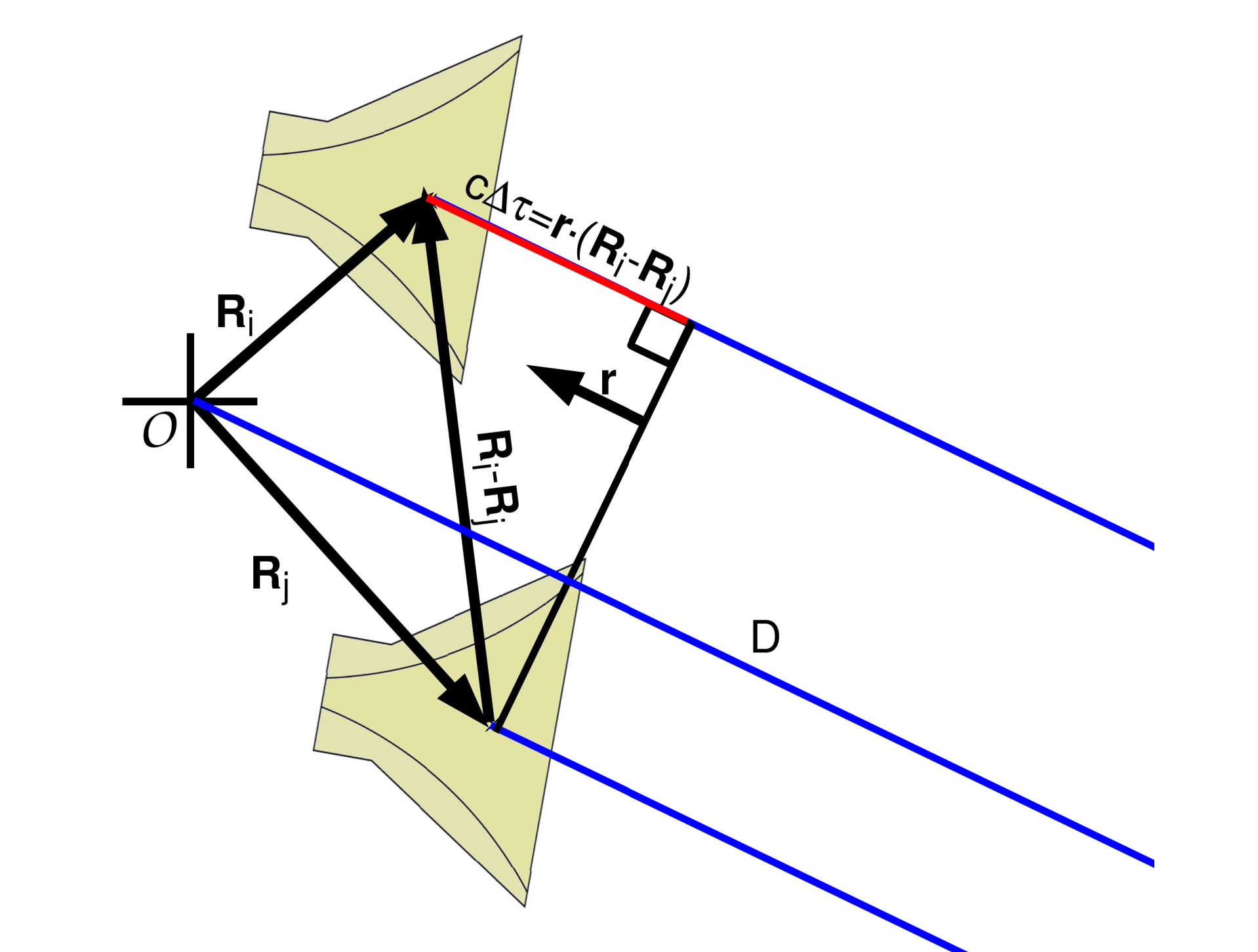
  1. The time delay between any antenna pair is computed via \( (\bf{X_1} - \bf{X_2}) \cdot \hat{\bf{u}} \) / \(c\)
     • \(\bf{X}\) denotes the antenna position,
     • \(\hat{\bf{u}}\) is a unit vector that represents the signal direction, and
     • \(c\) is the speed of light.
  2. Each entry in the column time delays [sec] would be a 2D matrix with the same dimensions as the 2D grid generated by _make_grid; let's call them time delay skymaps.
  3. Each point on a time delay skymap represents the expected time-delay based on where the signal is coming from and where the antennas are on the payload.
  4. Time delay occurs since the signal has to travel an extra distance to reach the second antenna, after it hits the first antenna:
     
  5. As an example, the figure below shows the expected time delays (in seconds) between antenna 203 and 104.

Time Delays of Signals from Different Directions

Definition at line 89 of file time_delays.py.